The VIX/SKEW matrix to build sharpe 2+ strategies.

Understanding supply and demand is all you need

The word skew generates so much fantasy in the trading psyche that I tried hard to avoid it. Yet, sometimes you have to call a cat a cat, as we say in French.

Today, we address one of the most fascinating features of the option market: the implied volatility surface.

It has two main components: the level of the surface, which, in business terms, translates to the general demand for options, and the skew, which, in business terms, shows the excess demand of puts versus calls.

It is well-documented that the price of out-of-the-money options is often, all else being equal, higher than the price of the at-the-money option. To put it in implied volatility terms, IV ATM is very often below IV OTM. The extent varies from the market context (type of asset, tickers, market regime).

I’ll avoid complicated theories and instead focus on the backbone of what we do: as traders, we buy and sell assets or contracts to other market participants. There is literally no difference between what you trade electronically on your phone and the fruits and vegetables market on your street corner.

Let’s meet there for the rest of this article.

A side note: If you expect many complicated derivatives equations and theories about dealers’ positioning, this article isn’t for you. However, if you are patient through the explanation, there is a nice trade at the end for the subscribers. There is currently a 46% discount on the house; do not miss it.

A story of AAPLs and oranges

Jose works hard to sell the apples from the family farm and puts his booth every Tuesday, Thursday, and Saturday morning at the center of the village. Some days, Jose can quickly pick up the fact that there won’t be much demand for his apples, so by 9 am, he starts dropping his prices: an apple sold at a lower price is better than an apple he has to return home with. Yet these are the same apples as yesterday or tomorrow. The only thing affecting their value is the supply and demand mechanism and not the underlying feature of the fruit.

We tend to forget this critical concept when we trade electronically; supply and demand are all you need. I am not talking about the flow and all the convoluted explanations around second-degree derivatives, dealer positioning, or, my personal favorite, the theories on who is the aggressor. Jose doesn’t care about any of that to make money. And it’s not because you trade on an iPhone 16max that you are a much more sophisticated trader than Jose.

Supply and demand affect the price of options the same way they affect apples and oranges on a Thursday morning at the street corner market. When there is a lot of demand for options, market makers will slightly tilt their quotes and carefully manage their inventory. They will sell at a discounted price if there is no excessive demand.

We haven’t mentioned Greeks, delta or gamma, or emotions like fear or euphoria: these are secondary-degree explanatory factors.

When Jose slightly raises his prices at 9 a.m. because he sees a lot of demand today, he isn’t asking himself whether apple buyers are concerned about a shortage of apples. He just reacted to the market.

The same thing applies to options. Market makers will raise their quotes because they see a lot of demand for their options, whatever the reason.

There is one problem, though—one day, Jose is busy selling many apples, but he can tell his friend John struggles with his oranges. Yet, the number of customers on the market is as high as ever, and when people buy apples, they usually buy oranges. So what’s up with them?

Generally speaking, how can we effectively and in real-time measure how strong the demand is and when to decide whether to increase prices?

Measuring the demand for options with raw prices and no BS (Black Scholes).

Comparing the price of your apple today versus the average price of apples over the past three months is a good starting point. Doing the same operation with oranges will paint a better picture of the situation Jose is witnessing: John is still drunk from yesterday, and his quotes are way too high. People are not interested in oranges anymore, and all of a sudden, the prices of apples … look much more appealing, hence why Jose has been able to increase his prices for the past hour. Once again, he reacted to pent-up demand generated by something happening in the marketplace.

That trivial example helps us build intuition around the critical concept of implied volatility. In the options market, excess demand is measured with implied volatility: market makers react and raise their prices when there is a lot of demand for options. To measure that excess demand, you must compare your options' current price to some benchmark. And what better benchmark than the underlying price itself?

One of the cleanest ways to measure implied volatility is to compare the current prices of all out-of-the-money options against the inherent value of the underlying. This method is clean because it makes no assumptions about how the market is supposed to behave—just raw prices and no B&S.

Spooky spooky - some hieroglyphs!

It turns out that there is an elegant, yet a bit intimidating, formula that does that really well—the VIX formula, which is nothing but a big weighted sum of out-of-the-money calls and puts prices based on how far from the money they are. There are additional normalization effects, particularly around time to expiration, to ensure that you can compare apples to apples or implied volatility to implied volatility.

Now, we can easily compare the implied volatility for AAPL, NVDA, and SPY without making strong assumptions about the distribution of their returns.

The VIX for these instruments is a good proxy for implied volatility.

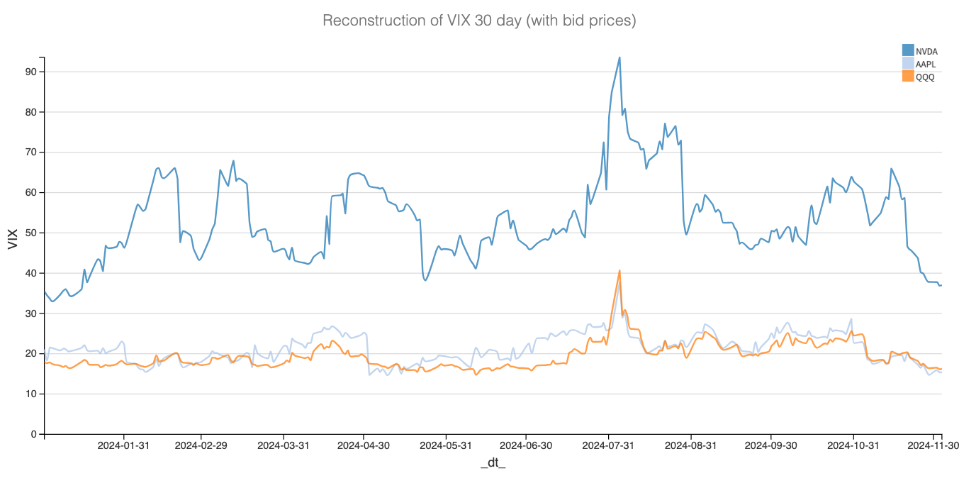
When that number is high, you can only conclude that the demand for options or implied volatility is high. When it is low, the demand for options is low.

Implied volatility needs market context to be relevant.

The chart above provides a concrete example: NVDA VIX is at 37 right now. The number sounds scary, but in the context of NVDA, it is at its lowest point this year. But AAPL VIX 37 this summer, yes, you had all the reason in the world to be concerned about a crash in AAPL.

But why exactly? As a reminder, implied volatility describes the general level of demand for every option. Because we sum up the price of all OTM puts and calls, just looking at that number, you can’t entirely conclude whether the prices of puts or calls drive the general level of demand. It is market-dependent.

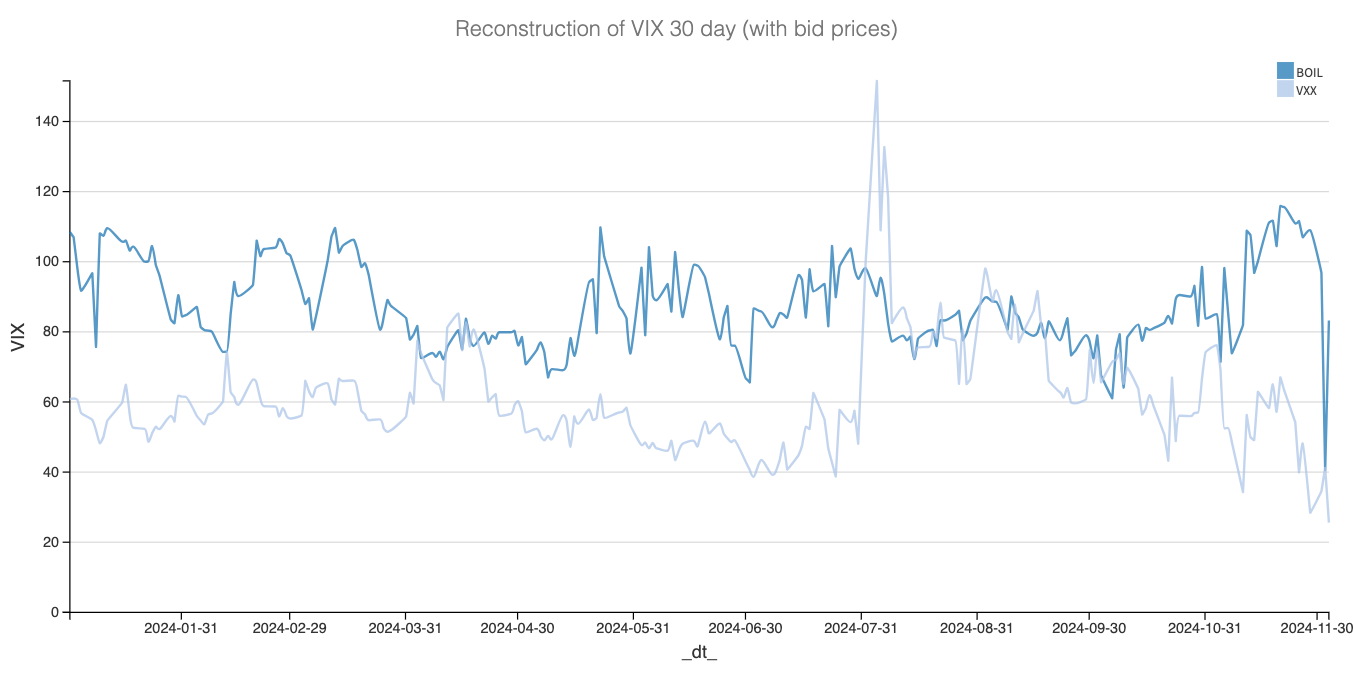
For instance, the implied volatility in BOIL is driven by calls, which is very different from NVDA, where puts drive it.

So when we hear analysts say the VIX is high, the market is fearful, and a crash is brewing, this is because we know that the price of puts primarily drives the VIX. But if I tell you tomorrow that the VIX on VXX is high, jumping to the conclusion that VXX is about to crash would make no sense.

BOIL and VXX call prices matter greatly on the implied volatility level. But it’s hard to tell from this chart unless you know how the underlyings behave.

Wouldn’t it be nice if we could compare the overall demand for puts versus the demand for calls?

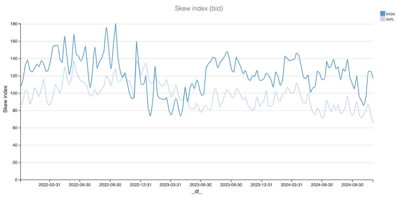
Skew enters the chat.

The skew, without shortcuts.

If you’ve followed up until then, the skew explanations, without any math formula, will be very intuitive.

If the general demand for options is a big sum of call prices AND put prices, the cleanest way to get a feel for the skew is to subtract call prices from put prices.

The demand for put is more pronounced in NVDA than in AAPL.

I can already hear some complaints—duh, K. All that lengthy explanation when you could have taken a 25 delta put and subtracted a 25 delta call and been done with it.”

That sentence in and of itself is the reason why traders can’t be great cooks: you must slow down and resist taking shortcuts.

First, we avoided the concept of delta and Greeks because it makes some questionable assumptions about market behaviors. It is helpful for many business cases, but not today.

Second, this simplification ignores a key issue—what if the price distortion starts much after the 25 delta? Why 25 and not 10? Why not 10 or 30?

Traders won’t have a better answer than “because it is practical or because we’ve already done it this way.” That is not enough to make a great recipe.

Let’s take a trivial example to build some intuition.

AAPL is at 100, and the trader uses the put 90 and the call 110 to get a feel for the skew. But it turns out that buyers have been hitting 85 puts all day, driving the price up. Your skew metric is … blind and skewed. It won’t consider the distortion happening below your strike of choice.

That’s why it’s worth taking all the prices of puts and subtracting them from the prices of all calls.

If the general demand is measured as the big sum of out-of-the-money calls and out-of-the-money puts, the skew is the difference between the Riemann sum of out-of-money puts and out-of-money calls. You can get fancier and more complicated, but this is a good compromise between the excessive precision quants often require and the dirty and pragmatic way of finding edges in the market.

Yes, because I didn’t write almost 1750 words about apples and oranges just for the sack of it.

Here is the edge.

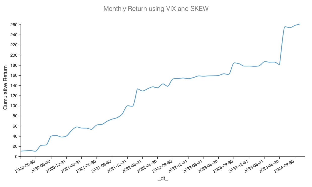
If you haven’t subscribed yet, now is your chance. There is a 46% discount at the moment, a bonus from the performance so far in 2024.